What is Robinhood?

Robinhood is a brokerage offering commission free trading. This is a big deal. Average online brokers charge between $4 and $12 per trade. These fees can really eat into your profits — especially for new investors with smaller portfolios.

In addition to the usual equity trades, Robinhood also offers services for options and crypto currencies with plans to continue expanding. Limited after hours trading is included, too! The zero-fee structure and multitude of offerings make Robinhood an attractive investment platform indeed.

Is it really free?

Yes, all trades are really commission free. You will pay no fees whatsoever to Robinhood.

Then how does Robinhood make money?

Well, several ways actually. That little bit of cash lying around while you wait for the right stock to buy? Similar to a bank, Robinhood will invest that cash for their own profit. This is the most widely reported tactic.

But… the above method is likely no more than a drop in the bucket for Robinhood. The real money is made through a process called Payment for Order Flow. This is when a brokerage sells transaction information in real time to high frequency trading firms. There is a lot of controversy around the issue as a whole. Interestingly, it was none other than Bernie Madoff that came up with the idea in the first place. Few liked the idea in principal, but none could resist the profitable temptation for long. Today, most brokerages all partake in the practice.

I was speaking with a professor just the other day who declared, “Robinhood is ripping all the millennials off.” After a short discourse, his real problem was not with Robinhood specifically, but with brokerages receiving payment for order flow. TD Ameritrade, Charles Schwab, and Vanguard all participate in this practice, just to name a few. If, like my professor, this is a deal breaker for you Interactive Brokers could be an alternative. In my opinion, order flow agreements should only enter the equation if you regularly buy thousands of shares at a time.

The final way Robinhood generates cash is with paid margin accounts. For a flat monthly fee, investors can receive up to 2x their normal buying power.

$2000 in margin for $10/month

Is Robinhood safe?

I’m going to consider “safe” in this context as the likelihood Robinhood is engaging in illegal activity. Obviously, all investments come with an amount of market risk.

I have no special insight, but I do believe Robinhood to be safe. I have had money invested with them since 2016 and have successfully sold, bought, deposited, and withdrawn cash with no surprises. Robinhood is also a member of FINRA, insured under SIPC. What’s that alphabet soup mean for you? Essentially, the Securities Investor Protection Corporation, a non-profit, has your back (up to $500,000). It’s very similar to the FDIC insurance from banks that people are more acquainted with. If Robinhood goes bankrupt for any reason, SIPC will kick in and ensure you receive your shares. There is one important difference, however. SIPC does not protect against illegal activity. If Robinhood knowingly defrauds investors, SIPC insurance is not applicable. While I believe the risk for this is near-zero, it’s a fact worth knowing.

Robinhood’s investors include Kleiner Perkins, Google Ventures, and even Snoop Dogg. So, if the executives take the money and run off to a non-extradition country, at least you’ll be in good company.

User Experience

Robinhood’s interface, while beautiful, lacks the more thorough information veteran investors are likely accustomed to. This can be easily remedied by researching on another platform and trading with Robinhood.

Don’t expect to be able to fine tune the graph either. Only the presets are available and it’s impossible to overlay multiple stocks, or other indicators to identify fundamentals like death crosses.

Customer support is also lacking. There is no phone number to call, no online chatroom to help. Support is restricted solely to email and can reportedly be a little on the slow side (Reddit link to unhappy customer). I have not had the need to contact them yet, so have no first hand experience to report.

What’s this buzz around cash management?

Recently, RH announced that a Cash Management service will be coming soon. They expect to offer 3% interest on the cash balance in your trading account and let you spend it via a debit card just like a regular checking account.

There is a pretty significant catch, however. Unlike a regular bank, these cash management accounts are not going to be FDIC insured. Originally, Robinhood claimed SIPC protection would apply, but SIPC President Stephen Harbeck quickly refuted their claim.

Until more information is released, it’s impossible to do more than speculate. For now, I’d recommend sticking with a high interest online savings account for collecting risk-free returns and using Robinhood for equities.

Time to take the plunge!

Overall, it’s a great platform for beginning investors or smaller balances that would otherwise be eaten away by trading fees. The compounding nature of investments means the best time to start was yesterday, but the second best time is today.

If you’ve decided to pull the trigger and invest with Robinhood, please consider using this referral link. We’ll both receive a free stock. I would never recommend a product I don’t use myself. I rely on Robinhood for the majority of my stock and options trading.

Still have questions? What’s your favorite brokerage? Let me know in the comments!

Altman Z Score – Determining Bankruptcy Probability with QuantConnect

The Altman Z-Score is an indicator used to determine a company’s likelihood of declaring bankruptcy. A total of five ratios are necessary for the calculation. Lucky for us, they are all readily available for public companies.

The Formula

Let:
A = Working Capital / Total Assets
B = Retained Earnings / Total Assets
C = Earnings Before Interest / Total Assets
D = Market Value of Equity / Total Liabilities
E = Sales / Total Assets

Then the Altman Z Score can be calculated by:
Z = 1.2A + 1.4B + 3.3C + 0.6D + 1.0E

The relative probability of default is determined by the Z value. Specifically,

Z ≥ 3 → Safe
1.81 ≤ Z < 3 → Warning
Z < 1.81 → Danger

Note that these cutoffs are from the original Altman Z Score. Different intervals have been derived for emerging markets. More information is available on Wikipedia.

Algorithm

This algorithm is heavily based on code from Aaron Gilman. It has been updated to work with new versions of QuantConnect.

It works through universe selection. Universe selection allows us to filter equities based on predefined search criteria. In this case, it selects equities that have 1) all the necessary data available for calculating the ratios and 2) a Z Score greater than 1.81. Next, the results are sorted by EBITDA and capital is equally divided among the top 100 equities. The portfolio is re-balanced on the first trading day each month.

Historic Accuracy

In Altman’s initial publication, the Altman Z Score was 72% accurate in predicting bankruptcy within two years. False negatives, however, were extremely low at just 6%. This initial accuracy has not only been proven, but actually found to be a conservative estimate. Over the years, Altman’s model was found to be 80-90% accurate — but with a higher false negative rate of around 15%.

Today, Altman’s Z Score is widely accepted. Originally designed for manufacturing companies with over $1 million in assets, it’s now used in a variety of countries and industries, though sometimes with slight modifications.

Caveats

As with most balance sheet models, the Alman Z Score should not be applied to financial companies. The balance sheets of Wallstreet companies are notoriously opaque and off-balance sheet items are numerous — making accurate calculations nearly impossible.

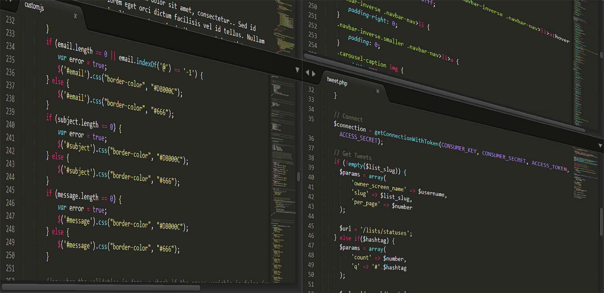
Building your first algorithm in QuantConnect (Python)

This post will guide you through developing your very own trading algorithm in QuantConnect. A familiarity in python and basic finance knowledge is assumed, but I’ll be gentle — promise! Already an expert? Skip to the code.

More comfortable with C#? View the alternate tutorial.

The algorithm we’ll build is based on the principle of a proportionated simple moving average (P-SMA). We will choose a benchmark (SPY in this example) and, based on its simple moving average, decide if the market will go up or down. If we predict the market will go up, we will invest in equities that provide fast growth but increased risk. Otherwise, we invest in safe assets, such as treasury bonds. Proportionated means the decision is not binary. For example, we may calculate 30% of our portfolio should be relatively risk-less and allocate 70% for high growth equities.

Time to code! Any algorithm in QuantConnect starts the same way:

class ProportionalSMAFast(QCAlgorithm):
    def Initialize(self):
        pass

First, we instantiate the class. The name can be anything you like, but it’s important to extend QCAlgorithm. Whenever an algorithm is started, Initialize is called exactly once and allows us to setup the properties of our algorithm. Let’s begin to flesh out initialize.

def Initialize(self):
    self.SetCash(10000)

    self.SetStartDate(2016,01,01)
    self.SetEndDate(2016,10,14)

    # Add all assets you plan on using later
    self.spy = self.AddEquity("SPY", Resolution.Daily).Symbol
    self.qqq = self.AddEquity("QQQ", Resolution.Daily).Symbol
    self.tlt = self.AddEquity("TLT", Resolution.Daily).Symbol
    self.agg = self.AddEquity("AGG", Resolution.Daily).Symbol

    self.benchmark = self.spy

    self.risk_on_symbols = [self.spy, self.qqq]
    self.risk_off_symbols = [self.tlt, self.agg]

Methods such as SetCash, SetStartDate, and SetEndDate are only applicable when running a back-test. They are completely ignored during live trading.

AddEquity is essential to any algorithm you write. By adding the equity in the initialize method, the relevant equity data will be made available throughout your algorithm. Resolution.Daily specifies data will be given with a daily window. Other options are tick, second, minute, and hour.

So what about the .Symbol and self.my_equity? Why assign the variable? This is not strictly necessary. Specifically, the following code is all that is required to make the equity data available.

self.AddEquity("SPY", Resolution.Daily)

By assigning self.spy, we can prevent hard coding the string "SPY" everywhere and use the variable instead. If you’re a little confused about this point, don’t worry. It will become more apparent later on.

And the final two lines? Remember, we want to invest in either high growth or low risk assets depending on the market. risk_on_symbols will be invested when we want to add risk to our portfolio — predicting an upswing. risk_off_symbols are our low risk investments. You should feel free to experiment with different symbols. You can add as many or as few equities as you like to either list.

#Schedule every day SPY is trading
self.Schedule.On(self.DateRules.EveryDay(), \
                 self.TimeRules.AfterMarketOpen(self.benchmark, 10), \
                 Action(self.EveryDayOnMarketOpen))

The snippet above will complete our Initialize method. This is the main driver of your algorithm. It schedules a method called EveryDayOnMarketOpen to run every day that SPY (our benchmark) is trading, 10 minutes after market open.

Since setup is over with, let’s move on to the heart of the algorithm by defining EveryDayOnMarketOpen.

def EveryDayOnMarketOpen(self):
    #Do nothing if outstanding orders exist
    if self.Transactions.GetOpenOrders():
        return

Nothing groundbreaking here. We just return immediately if there are any open orders. In theory, this should never happen. Our algorithm will submit market orders 10 minutes after market open, and is run once per trading day. If this block does execute, it’s likely an indicator of a more serious, underlying problem. Nevertheless, better safe than sorry.

#Lookup last 84 days
slices = self.History(self.spy, 84)
#Get close of last (yesterday's) slice
spy_close = slices["close"][-1]

#Get mean over last 21 days
spy_prices_short = slices["close"][-21:]
spy_mean_short = spy_prices_short.mean()

#Get mean over last 84 days
spy_prices_long = slices["close"]
spy_mean_long = spy_prices_long.mean()

The self.History method returns a pandas data frame, representing data on the specified equity for the previous 84 days. Our algorithm compares moving averages over two different window sizes, 21 and 84 days. These are arbitrary (but common) intervals. I encourage you to experiment by changing these values. The next two blocks splice the last 21 and 84 closing prices from the data frame and calculate the average.

risk_on_pct  = (spy_mean_short/spy_close) * \
               ((spy_mean_short *2 / spy_mean_long) *.25) / \
               len(self.risk_on_symbols)
risk_off_pct = (spy_close/spy_mean_short) * \
               ((spy_mean_long *2 / spy_mean_short) *.25) / \
               len(self.risk_off_symbols)

#Submit orders
for sid in self.risk_on_symbols:
    self.SetHoldings(sid, risk_on_pct)
for sid in self.risk_off_symbols:
    self.SetHoldings(sid, risk_off_pct)

Finally, the exciting stuff! The “risk on” and “risk off” percentages are calculated using our history data. self.SetHoldings will allocate a percentage of your portfolio to the specified equity. For instance, self.SetHoldings("SPY", 1) will buy as much SPY as you can afford, 100% of your portfolio. If you have a margin account and want to leverage your position, simply allocate more than 100%. self.SetHoldings("SPY", 2) will buy twice as many SPY shares as you can actually afford.

That’s it! You now have an algorithm that can trade automatically on your behalf. I encourage you to experiment changing/improving the algorithm on your own.

This example is also available on GitHub.

Building your first algorithm in QuantConnect (C#)

This post will guide you through developing your very own trading algorithm in QuantConnect. A familiarity in C# and basic finance knowledge is assumed, but I’ll be gentle — promise! Already an expert? Skip to the code.

More comfortable with Python? View the alternate tutorial.

The algorithm we’ll build is based on the principle of a proportionated simple moving average (P-SMA). We will choose a benchmark (SPY in this example) and, based on its simple moving average, decide if the market will go up or down. If we predict the market will go up, we will invest in equities that provide fast growth but increased risk. Otherwise, we invest in safe assets, such as treasury bonds. Proportionated means the decision is not binary. For example, we may calculate 30% of our portfolio should be relatively risk-less and allocate 70% for high growth equities.

Time to code! Any algorithm in QuantConnect starts the same way:

namespace QuantConnect.Algorithm.CSharp{
    public class ProportionalSimpleMovingAverage : QCAlgorithm{
        public override void Initialize(){
            return;
        }
    }
}

First, we instantiate the class. The name can be anything you like, but it’s important to extend QCAlgorithm. Whenever an algorithm is started, Initialize is called exactly once and allows us to setup the properties of our algorithm. First, we’ll define some member variables. This should go immediately before Initialize, inside the class.

...
private static Symbol _spy = QuantConnect.Symbol.Create("SPY", SecurityType.Equity, Market.USA);
private static Symbol _qqq = QuantConnect.Symbol.Create("QQQ", SecurityType.Equity, Market.USA);
private static Symbol _tlt = QuantConnect.Symbol.Create("TLT", SecurityType.Equity, Market.USA);
private static Symbol _agg = QuantConnect.Symbol.Create("AGG", SecurityType.Equity, Market.USA);
   
private Symbol _benchmark = _spy;
   
private List<Symbol> _risk_on_symbols = new List<Symbol>{
    _spy,
    _qqq
};  
private List<Symbol> _risk_off_symbols = new List<Symbol>{
    _tlt,
    _agg
};  
   
private RollingWindow<decimal> _close_window;

public override void Initialize(){
    ...

When coding in C#, a common convention is to denote member variables with an underscore. The first four lines create the “symbol”, a reference to specify the desired equity. Next, we define our “benchmark”. This is the equity that will be used as the basis for all future calculations. Moving on to the lists: remember, we want to invest in either high growth or low risk assets depending on the market. _risk_on_symbols will be invested when we want to add risk to our portfolio — predicting an upswing. _risk_off_symbols are our low risk investments. You should feel free to experiment with different symbols. You can add as many or as few equities as you like to either list. The final member variable is_close_window. This is a rolling window — a special list that will only keep a fixed number of the most recent elements. Specifically, we’ll be using a window size of 84, and storing decimal numbers (daily closing price of the benchmark equity); because the window is not static, we declare it here but instantiate the window later inside the Initialize method.

Let’s begin to flesh out initialize.

public override void Initialize(){
    SetStartDate(2016, 01, 01);
    SetEndDate(2016, 10, 14);
    SetCash(10000);

    AddEquity(_spy, Resolution.Daily);
    AddEquity(_qqq, Resolution.Daily);
    AddEquity(_tlt, Resolution.Daily);
    AddEquity(_agg, Resolution.Daily);
}

Methods such as SetCash, SetStartDate, and SetEndDate are only applicable when running a back-test. They are completely ignored during live trading.

AddEquity is essential to any algorithm. By adding the equity in the initialize method, the relevant information will be made available throughout the algorithm. Resolution.Daily specifies data will be given with a daily window. Other options are tick, second, minute, and hour.

_close_window = new RollingWindow<decimal>(84);
IEnumerable<TradeBar> slices = History(_benchmark, 84);
foreach(TradeBar bar in slices){
    _close_window.Add(bar.Close);
}

The code here is responsible for initializing the rolling window. The first line creates the window and sets the type and size to decimal and 84 respectively. Next the History function is called to get historical information about the benchmark during the last 84 days. Finally, we loop through every day of historic data and add the closing price to the rolling window. This ensures the algorithm will always have 84 days of information to use for calculations.

Schedule.On(DateRules.EveryDay(_benchmark),
        TimeRules.AfterMarketOpen(_benchmark, 10),
        EveryDayOnMarketOpen);

The snippet above will complete our Initialize method. This is the main driver of your algorithm. It schedules a method called EveryDayOnMarketOpen to run every day that SPY (the benchmark) is trading, 10 minutes after market open.

Next, we build a simple function to assist with calculating averages over various window sizes.

private decimal GetRollingAverage(int n, RollingWindow<decimal> window){
    decimal sum = 0;
    for (int i = 0; i < n; i++){
        sum += window[i];
    }  
       
    return sum / n;
}

This function accepts two parameters, an integer n denotes the number of days to look back, and a RollingWindow over which to do the averaging. The for loop will iterate through the window until it reaches the nth entry. At that point, the sum will be divided by n and the simple average will be returned.

Since setup is over with, let’s move on to the heart of the algorithm by defining EveryDayOnMarketOpen.

public void EveryDayOnMarketOpen(){
    if (Transactions.GetOpenOrders().Count > 0){
        return;
    }  
}

Nothing groundbreaking here. We just return immediately if there are any open orders. In theory, this should never happen. Our algorithm will submit market orders 10 minutes after market open, and is run once per trading day. If this block does execute, it’s likely an indicator of a more serious, underlying problem. Nevertheless, better safe than sorry.

IEnumerable<TradeBar> slices = History(_benchmark, 1);
TradeBar last_bar = slices.Last();
decimal bench_close = last_bar.Close;
       
_close_window.Add(bench_close);
       
decimal bench_mean_short = GetRollingAverage(21, _close_window);
decimal bench_mean_long = GetRollingAverage(84, _close_window);

The History method returns TradeBars, representing data on the specified equity. We use the History function to get yesterday’s closing price and add it to the rolling window. The final two lines calculate the average closing price over the specified period. Our algorithm compares moving averages over two different window sizes, 21 and 84 days. These are arbitrary (but common) intervals. I encourage you to experiment by changing these values. Note that if you want to look back past 84 days the rolling window size will need to be increased in the Initialize function. QuantConnect does offer convenience methods to calculate various indicators to use in your projects, which makes code easier to read.

decimal risk_on_pct = (bench_mean_short / bench_close) *
                        ((bench_mean_short * 2m / bench_mean_long) * .25m) /
                        _risk_on_symbols.Count;
decimal risk_off_pct = (bench_close / bench_mean_short) *
                        ((bench_mean_long * 2m / bench_mean_short) * .25m) /
                        _risk_off_symbols.Count;

foreach (Symbol sid in _risk_on_symbols){
    SetHoldings(sid, risk_on_pct);
}  
foreach (Symbol sid in _risk_off_symbols){
    SetHoldings(sid, risk_off_pct);
}

Finally, the exciting stuff! The “risk on” and “risk off” percentages are calculated using our history data. SetHoldings will allocate a percentage of your portfolio to the specified equity. For instance, SetHoldings(_spy, 1) will buy as much SPY as you can afford, 100% of your portfolio. If you have a margin account and want to leverage your position, simply allocate more than 100%. SetHoldings(_spy, 2) will buy twice as many SPY shares as you can actually afford.

That’s it! You now have an algorithm that can trade automatically on your behalf. I encourage you to experiment changing/improving the algorithm on your own.

This example is also available on GitHub.

What is QuantConnect? A review.

Anyone with a strong interest in finance will eventually hear of “quants” — the mystical math prodigies behind many of the trades on Wall Street today. While Quantitative Analysts come in a few varieties, I find algorithmic traders the most exciting. They’re responsible for crafting sophisticated computer programs to automatically trade equities, currencies, futures, and really anything and everything else that can turn a profit. Traditionally, having the resources to trade live — with real money — has been restricted to multi-million (or billion) dollar hedge funds. QuantConnect is a platform that allows anyone to create live trading algorithms.

This means you can connect your Interactive Brokers/E-Trade/Gdax/whatever account to QuantConnect and build a simple program to trade on your behalf. Hell, you might create the next cutting-edge innovation, license it to a company for millions, and retire in the Caribbean.

So, without further ado: a hands on review on QuantConnect.

Interface

Three languages are available: C#, Python, and F#

The online IDE is intuitive. Upon starting an algorithm, three programming options are available: C#, Python, and F#. Initially, I felt the abundance of language options to be frivolous, but now I can’t imagine any other way. Find a great library in C# you’d like to add? Want to code some ML with SKLearn in Python? No problem. What really stands out is the ability to add multiple files. This is an enormous help when developing complex algorithms or importing third party libraries. It replicates a more natural coding environment without the usual limitations of an online interface.

Must-haves such as syntax highlighting and auto complete work brilliantly. Most of the time the prompt is automatic. Just like other IDEs, it can be manually invoked with Ctrl + Space.

Autocomplete works as expected

Still not a fan of developing in a web browser? Since the framework that runs QC is open source, it’s a breeze to get it running locally so you can use visual studio (or vim) — which is a good thing, because you’ll probably need it. As capable as the system is, it falls short on debugging. There is no interactive debugger, so you’ll be stuck relying on error messages that look like this:

BacktestingRealTimeHandler.Run(): There was an error in a
scheduled event EveryDay: SPY: 10 min after MarketOpen. The error was
Python.Runtime.PythonException: NameError : global name 'foobar' is not
defined

Notice something missing? There’s no line number! Leaving you stuck guessing exactly where the flaw lies. I should mention, this is only a problem with runtime errors. Any problems during compilation will be flagged and the line number identified.

Algorithms can be shared with email or account name

Collaborating with a friend? QC makes this a breeze. Simply hit share and you can work in tandem. Want to rename, move, or delete a project? All actions are as expected.

Overall, the interface does it’s job very well.

Speed

There’s two important aspects to “speed” during algorithm development. The time a backtest takes to complete, and the delay before receiving live data.

Backtesting speed is comparable to any other platform. You might expect to see large differences between an algorithm programmed in C# and an algorithm in Python. Empirical evidence suggests this is not the case. Runtimes were nearly identical across languages.

Language Average Time
C# 6.183333333
Python 6.76666666

Occasionally, there has been a wait time before starting a backtest; indicated in the results chart. This can be very annoying when trying to meet a deadline — but in my experience it’s a rare enough occurrence to not be a concern.

Results tab displays a wait time of 12

QuantConnect advertises co-located servers with minimal delay. A post from the founder on Reddit suggests speeds between 20 and 100ms. This may not be directly competitive with Wall Street firms, but it far exceeds any competition available for personal accounts. The delay is enough to be prohibitive for very high frequency trades, but is still impressive. Note that we took QuantConnect on their word here. These times were not tested.

Community

Small but mighty! In my experience, searching alone will seldom solve your problem — but people are happy to help. Posting a specific question on the forum typically yields a quick response. The QuantConnect team is also very active and helpful. They go as far as to offer free code reviews to interested users.

Price

If you’re only looking for a research platform, the price can be free. However, if you have absolutely no interest in live trading, there are plenty of alternatives. To take advantage of where QC really excels, the price starts at $20/month. Depending on the size of your portfolio, that may sound too good to be true, or a little steep. However, I’m confident even rather small portfolios will more than make up for the price with a good algorithm.

The real expense happens if you want to run multiple algorithms simultaneously. Each algorithm runs on its own, isolated VPS. This creates large reliability and performance benefits, but comes at a cost. Every additional algorithm is an added $10.

Bonus features

One unique feature QC has to offer is version control. Every time an algorithm is backtested, a snapshot is created. This allows for development without worry — knowing you can revert to a previous version at any time.

Alternatives

Quantopian, once a fierce competitor, has suspended all live trading. It is still a capable research platform, if you’re willing to forgo trading with real money.

IBridgePy is a self-hosted solution compatible with Interactive Brokers.

Most other alternatives are inaccessible to the average investor and targeted towards hedge funds. AlgoTrader is a prime example.

Bottom Line

QuantConnect is not without its problems — no platform is. However, it far exceeds anything offered by the competition and is improving everyday. At a competitive price with a tremendous staff, no one else comes close.

Oh, and if you do end up retired under 30, sipping Piña Colladas by the beach — don’t forget about the blogger that helped get you there. 🙂

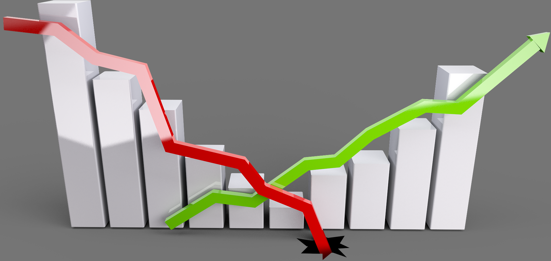
Death Cross – QuantConnect Algorithm

Death crosses are useful as trailing indicators. Specifically, a death cross occurs when the long term moving average passes above the short term moving average. The graph below depicts a death cross, highlighted in pink. It is a sign that the security is likely to fall in value.

Graph showing example of a death cross
Chart generated from bigcharts.com

Intuitively, this makes sense. The moving average is a trend over time. If the short term moving average falls below the long term moving average, it’s an indicator something has recently changed — for the worse.

Like any indicator, a death cross is far from foolproof. Since it’s a lagging indicator, if the downturn is short lived, by the time the indicator forms, the equity may have resumed an upward trend. In this instance, acting on the death cross is disadvantageous to the investor.

The opposite of a death cross is a golden cross. That is, a golden cross occurs if the short term moving average crosses above the long term average. A golden cross appears in the graph above in early August and is a sign of an upward trend.

Below are the results of a simple algorithm using death and golden crosses. The algorithm will go long on a golden cross and liquidate on a death cross.

Crosses really shine when used in conjunction with other indicators. The performance of crosses alone is far from groundbreaking.

Feel free to modify the algorithm on QuantConnect (GitHub). Changing the slow/fast period or symbol is a good place to start.

Have any algorithms that use crosses? A burning question I neglected to answer? Let me know in the comments!